Why is my VLOOKUP not working? - Four Opportunities To Improve Your VLOOKUP

This past week at a client site, I was asked a question that I have heard numerous times: Why is my VLOOKUP not working? I have seen issues with all of the four arguments required by this function and each presents an opportunity to improve your data model.

lookup_value

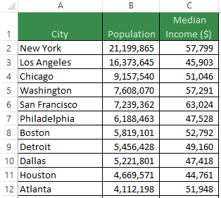I will keep the data set simple: population and median income for each city in the United States. This data set contains 503 cities.

Elsewhere in this spreadsheet, we need to lookup the population and median income of two cities: Buffalo and Hartford.

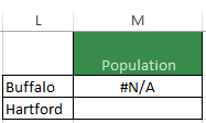
The text “Buffalo” is located in cell L2 and the VLOOKUP function to lookup the population will be written in cell M2.

The formula can be written as:
=VLOOKUP(L2,A2:C504,2,FALSE)

The first argument in the function is the lookup_value and represents what we want to look for. In this case we are looking for “Buffalo” which is in cell L2.

The second argument is table_array and represents the data source for retrieving the population of Buffalo. The table_array is in cells A2 to C504.

The third argument is col_index_num and represents which column in the table_array to return as our result. The population is in the second column, so we specify a value of 2.

The fourth argument is range_lookup and accepts values of TRUE (1) or FALSE (0). FALSE is “exact match” and only allows an exact match of Buffalo to return a result. TRUE is “approximate match” and will return the closest value to Buffalo if the table_array is sorted in the first column (City, from A to Z).

Here is the result of the formula, an #N/A error. The problem is that in cell L2, there is a space character after “Buffalo”. This is a common problem that is harder to find when many VLOOKUP functions are written. An easy way to resolve this issue in the lookup_value argument is with the TRIM function, which will remove all spaces from a string except for single spaces between words. The formula should be rewritten as:
=VLOOKUP(TRIM(L2),A2:C504,2,FALSE)


table_array

This formula in cell M2 can now be copied and pasted down one cell to M3. The resulting formula is:
=VLOOKUP(TRIM(L3),A3:C505,2,FALSE)

This formula returns the correct result for Hartford, but the table_array is no longer correct. The data source is now cells A3 to C505. New York is no longer in the table_array and every time this formula gets pasted one row further down, another city will be removed. To improve the table_array argument, add $ symbols to make it an absolute reference.
=VLOOKUP(TRIM(L3),$A$2:$C$504,2,FALSE)

Now the table_array will always remain the same. Unfortunately, if you add data to the bottom of the table starting in row 505, it won’t be visible to the function. Therefore, another way to write this formula is by using entire columns instead of specifying rows:
=VLOOKUP(TRIM(L3),$A:$C,2,FALSE)

This formula will copy and paste downwards without losing any data and also allows the data to grow.

col_index_num

The third argument is typically hardcoded as a number, in our case the second column is represented by a 2. There are two common issues created by hardcoding column references.

The first issue is what happens when you insert a column inside your table_array cell range. The State for each city has been added to the data and the Population is no longer in column 2, it is now in column 3. Excel does not update the VLOOKUP function because the col_index_num argument has been hardcoded. The Population lookup is now returning State instead because that is what appears in column 2.

The second issue is what happens when you copy and paste the formula in cell M2 to the right. If we want to add a VLOOKUP of Median Income in column N then we should add a $ symbol to the lookup_value ($L2):
=VLOOKUP(TRIM($L2),$A:$C,2,FALSE).


When this formula is copied and pasted to the right, nothing in the formula changes, so we have to manually change the col_index_num to 3. If we had more columns in our table_array such as Crime Rate or Unemployment Rate, we would copy and paste this formula to the right two more times and have to manually enter the col_index_num. For dozens of columns, this takes too long and is a risk for errors.

To fortify the col_index_num argument and solve both of these issues, use the COLUMNS function, which will count the number of columns in the cell range it is fed.

Replace the hardcoded value of 2 in the col_index_num argument with COLUMNS($A2:B2) which will evaluate to 2 (the number of columns in the range $A2:B2). The lookup in cell M2 for Buffalo’s population should be: =VLOOKUP(TRIM($L2),$A:$C,COLUMNS($A2:B2),FALSE)

When this formula is copied and pasted to the right, it becomes
=VLOOKUP(TRIM($L2),$A:$C,COLUMNS($A2:C2),FALSE) and the col_index_num now evaluates to 3. The range expands when pasted to the right. Furthermore, when the State column is inserted into the table_array, the col_index_num will also expand and return the correct result.

range_lookup

For just a few VLOOKUP functions, I would recommend using exact match (FALSE or 0) for the range_lookup argument because successful lookups will return the correct result and if the city is not found, an #N/A error is returned. However, if there are thousands of VLOOKUP functions in a data model and the table_array has a large number of rows, it will take a long time to recalculate the workbook. A significant performance boost is achieved by changing the range_lookup argument to approximate match (TRUE or 1). In order to do this, you must sort your table_array by the first column (City) and be sure that Buffalo appears in the table, otherwise you will return the population of the closest alphabetical match to Buffalo which may be Boston.

If you are interested in learning more about strengthening your data models, need a database solution or analytics training, please contact Scott Cuthbertson:

Email: scottjcuthbertson@gmail.com
LinkedIn: http://ca.linkedin.com/in/scottcuthbertson
Blog: http://theanalyticspro.blogspot.ca/

Scott Cuthbertson BBA

Scott is an Analytics Professional who has worked with over 100 clients in the retail and financial services industries. He has helped organizations improve their labour scheduling, inventory replenishment, performance management, organization design and pricing. He has been a practitioner of analytics since childhood, using data models to win Hockey Pools. His expertise lies in developing data models, reporting, algorithms and solutions for any organization that wants to use their data to improve decision making. He also teaches at the CMA Professional Development Institute.

© Scott Cuthbertson 2014 Blog: Words From The Analytics Pro