Simulation In Data Models - Introduce Uncertainty Into Your Life

When data models are built in Excel, assumptions are usually made. For example, take a look at this simple income statement data model (values are in thousands of dollars) and the associated calculations.

Revenue by region is fixed, the Cost of Goods are a percentage of Revenue and Overhead Expenses are fixed.

This model represents a forecast of a company’s Earnings for next year. It is static, so the result is always $170,000.

If this is a best guess at a forecast then the next level is to understand the possible variability in the model’s assumptions and results. How sensitive are Earnings to changes in Revenue?

Random Numbers

Random numbers can be used to add uncertainty to the data model. Even though Canadian Revenue is forecasted at $2,000,000, the worst case scenario is $1,500,000 and the best case scenario is $2,500,000. To reflect this in the data model, a random number in this range can be used instead of hard-coding $2,000,000. There are two common ways to implement this uncertainty in Excel:

=RANDBETWEEN(1500,2500)
=1500+RAND()*1000

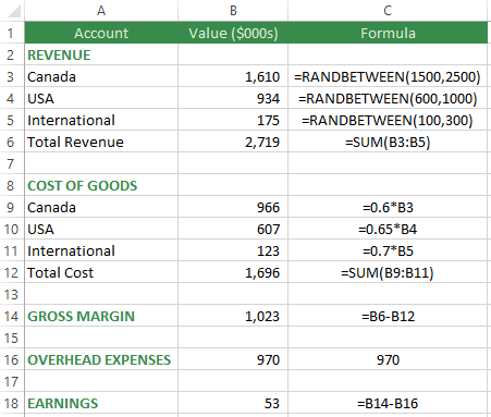
The RANDBETWEEN Function in Excel will randomly select a number within the range specified, including the lower and upper limits provided. Press the F9 key to trigger a recalculation of the Workbook.

The RAND() Function generates a random number between 0 and 1 (includes 0 but not 1). This value can be multiplied by 1,000 and added to 1,500 to generate a random number between 1,500 and 2,500.

USA and International revenue can also incorporate uncertainty in their values. USA revenue will range from $600,000 to $1,000,000. International revenue will range from $100,000 to $300,000.

Simulation: An Unorthodox Use Of Data Tables

Every time the F9 key is pressed, a recalculation of the Workbook will occur but the new scenario is not being captured. In order to capture the results from each scenario, you can use Visual Basic for Applications (VBA) code, but an easier way to capture the results is to use Data Tables.

Data tables are conventionally used to substitute a value from the first column in the table into a model parameter input cell in order to change the model and capture its result. However, in simulations, data tables can be used simply to trigger a recalculation of the same model and capture the result.

To set up the data table in this example, there is a formula in cell F2 (=B18) set to the model output: Earnings. Starting on the next row, one column to the left, fill down the number of scenarios desired. In this example I would like 10,000 scenarios. Next, highlight the top row and the rest of the table down to the last scenario. From the Excel Data ribbon, look in the Data Tools group and select What-If Analysis then Data Table.

Typically, when the Data Table dialog appears, the Column input cell (column of 10,000 values) is set to a cell in the data model where the numbers 1 to 10,000 will be placed before a recalculation, but in this case, all we want is a recalculation, so select a blank cell such as $S$17. Each of the 10,000 values will be placed in cell $S$17, forcing a recalculation, then then result at the top of the Data Table (cell F2) will be captured in each row below. Click OK to run 10,000 scenarios of the data model and capture each Earnings value.

Understanding The Distribution Of Model Results

In order to understand the results, first copy and paste the Data Table as values so they will not change on the next recalculation. Next, sort the Earnings from lowest to highest. With the sorted range selected, create a Line Chart to show how the simulation results are distributed. The chart shows that there are about 900 of 10,000 scenarios where Earnings are negative, which corresponds to a 9% chance of losing money based on the current model assumptions. If the target Earnings are $300,000, we can see that about 17% of the 10,000 scenarios yielded a value of $300,000 or greater.

These concepts are even more powerful with larger data models. Also, simulation can also use bell-shaped or other distributions instead of a simple RANDBETWEEN Function. Simulation is about understanding how sensitive results are to changes in assumptions. This allows the modeller to assign probabilities to the likelihood of scenarios and take action early to change the outcome.

If you are interested in learning more about Excel Data Model Simulation, let me show your organization how it can introduce uncertainty into its Excel models. If you need a data model, database solution or analytics training, please contact:

Email: scottjcuthbertson@gmail.com
LinkedIn: http://ca.linkedin.com/in/scottcuthbertson
Blog: http://theanalyticspro.blogspot.ca/

Scott Cuthbertson BBA

Scott is an Analytics Professional who has worked with over 100 clients in the retail and financial services industries. He has helped organizations improve their labour scheduling, inventory replenishment, performance management, organization design and pricing. He has been a practitioner of analytics since childhood, using data models to win Hockey Pools. His expertise lies in developing data models, reporting, algorithms and solutions for any organization that wants to use their data to improve decision making. He also teaches at the CMA Professional Development Institute.

© Scott Cuthbertson 2014 Blog: Words From The Analytics Pro

Ctrl+Shift+Enter - Welcome To The Wild World Of Excel Arrays

One of the most obscure and least documented features in Excel is also one of the most powerful. If you have not yet encountered array calculations in Excel, I’ll let you in on the secret. An array formula is one that performs multiple calculations in one cell. Here is a simple example:

In order to calculate the value of inventory, the Cost should be multiplied by the Units On-Hand for each Item. Once the four multiplications have taken place, the results should be summed.

A common approach to this calculation is to add a new column to perform the multiplications. The formula in cell D2 is =B2*C2, in cell D3 is =B3*C3, and so on.

After each row’s Cost Value is calculated, a SUM Function adding column D will total $97.00. This result was obtained in two steps and used five cells, one for each Item and one for the SUM. If there is more data, this approach will use more cells to calculate a result. The accumulation of enough of these intermediate calculations can bloat a data model to a size that is difficult to open or email.

An Array Formula can achieve the same result of $97.00 by performing this calculation in one step using one cell. The Array Formula is: =SUM(B2:B5*C2:C5)

Each of the four cells in column B is multiplied by the corresponding cell in column C. The four multiplications are then enclosed in a SUM Function to add the four results. The only problem is that after typing in this formula and pressing the Enter key, a #VALUE! error appears. Since this formula is an array calculation, it needs to be entered using a special combination of keys: Ctrl+Shift+Enter. Hold Ctrl and Shift down while pressing Enter, doing this will enclose the formula in curly brackets. This is Excel’s method of showing that it understands that an array operation is performed. The curly brackets are never typed in, they result from entering an array formula with Ctrl+Shift+Enter.

There is another Array solution for this calculation that does not require Ctrl+Shift+Enter, the SUMPRODUCT Function. You can see in the function ScreenTip that an array is expected. =SUMPRODUCT(B2:B5,C2:C5) and then Enter will multiply corresponding cells then add the results. Ctrl+Shift+Enter was required in the previous example because the SUM function is not expecting arrays to be multiplied inside.

This example is a simple introduction to the existence of array calculations. The real benefit of an array formula is in situations where there are thousands of Items. The array formula can be performed in one cell without the need for thousands of intermediate calculations. This results in smaller data models and can help avoid 30-60 Megabyte file sizes.

Also, array formulae open up amazing new possibilities…

Where is the MAXIF Function? Where is the MINIF Function?

A common gateway to the world of array calculations is when you want to retrieve the maximum value based on a condition, a MAXIF function. Even though Excel has provided functions for SUMIF, COUNTIF and even AVERAGEIF, there is no MAXIF. Here is an example to show how an array formula can simulate MAXIF until the day when Microsoft adds the MAXIF function to Excel.

This data set stores the sales value for each salesperson on each day through the year. Imagine the table starts in cell A1 and ends in cell C2000. What is the largest daily sales value for Tara? The solutions I see most often are:

1) Manually sort or filter the data to calculate the MAX Function for the “Tara” records. This is a good solution for a quick one-time calculation but is not ideal for calculating the MAX for each salesperson.

2) In column D, add an IF Function for each row to only display sales values where the salesperson is “Tara” then use the MAX Function on the new column. This solution is not much better than the first one.

3) Use a PivotTable to calculate the MAX value for Tara and the other salespeople. This is a good solution and has much more flexibility than the first two.

4) Use an array formula for maximum flexibility.

I prefer formula-based solutions because they automatically recalculate when cell inputs change. Here is the array formula to calculate Tara’s maximum daily sales (don’t forget Ctrl+Shift+Enter):

=MAX(IF($B$2:$B$2000=E2,$C$2:$C$2000,""))

IF($B$2:$B$2000=E2,$C$2:$C$2000,"") will perform 1,999 IF calculations, each comparing a value in column B to “Tara” in cell E2. Wherever the column B value is “Tara”, the corresponding value in column C is returned, otherwise the empty string “” is returned. Once all these IF calculations are finished, they are enclosed inside a MAX Function which will extract the largest value. The spreadsheet has been spared the use of 1,999 cells.

This formula can easily be copied and pasted downwards to the other salespeople. The formula can also be easily modified to determine the MIN, MEDIAN or QUARTILE of Tara’s sales values. Any summary function can be used to quickly understand the data.

One caution though, since almost 2,000 calculations are happening in one cell, the array formula takes a little longer to calculate than a simple formula, but only one cell was required. It is not advisable to take this array calculation and copy and paste it thousands of times, you will have wandered into the realm of databases at that point.

Knowing how to use arrays will take your data models to the next level of efficiency. Array calculations work in different versions of Excel and can help you create better data models. There are many more applications of these ideas, especially those simulating database functionality on a small scale in Excel.

If you are interested in learning more about Excel Array Calculations, let me show your organization how it can improve its Excel models. For any analytics training or analytical solutions, please contact:

Email: scottjcuthbertson@gmail.com
LinkedIn: http://ca.linkedin.com/in/scottcuthbertson
Blog: http://theanalyticspro.blogspot.ca/

Scott Cuthbertson BBA

Scott is an Analytics Professional who has worked with over 100 clients in the retail and financial services industries. He has helped organizations improve their labour scheduling, inventory replenishment, performance management, organization design and pricing. He has been a practitioner of analytics since childhood, using data models to win Hockey Pools. His expertise lies in developing data models, reporting, algorithms and solutions for any organization that wants to use their data to improve decision making. He also teaches at the CMA Professional Development Institute.

© Scott Cuthbertson 2014 Blog: Words From The Analytics Pro

Reclaim Your Weekend With Excel VBA - Three Common Repetitive Tasks To Automate

Whenever I mention “VBA”, business professionals tremble at the thought of programming code. However, I believe that a little coding ability is the next frontier for those who need to transform data into information to generate insights and make decisions. Coding is not exclusively the domain of developers and technology professionals. Business professionals can achieve 80% of the benefits by knowing 20% of the code. Since Microsoft Excel is the world’s most popular analytics tool, it makes a lot of sense to introduce coding using this comfortable environment.

When I was unfamiliar with Excel VBA (Visual Basic for Applications), I was working weekends in order to compile, clean, validate and finally analyze the data I was given. Fifteen years later, I automate the repetitive processes and devote most of my time to asking questions about the data and looking for the answers. I have seen countless colleagues struggle to analyze data because it never seems to arrive in a desirable format, so a lot of time is spent preparing data for analysis and much less time is spent performing analysis. My best experiences have been 5% data preparation and 95% analyzing the data to uncover the best questions and insights.

Investing a little time to learn how to automate a repetitive process will save you much more time in the long run. If you find yourself repeating the same tasks over and over, it can be automated. Here are three common time consuming problems in Excel data analysis and solutions that use Excel VBA.

“Unpivoting” Data

It amazes me how much data arrives in the following format:

This data is really a report which displays sales for each store (rows) and each week (columns). The format can be described as cross-tabulated or pivoted. I never recommend doing data analysis using this format because it is more difficult to manipulate than the exact same dataset in the following format:

The data to the left is “unpivoted” and is ideal for sorting, filtering and aggregating. I figure that business professionals naturally have a preference for this format because I am often asked to “unpivot” their data table.

If the dataset is small, then it won’t take too long to rearrange the cells manually, but how about hundreds of rows and columns? Automation is even more important if this needs to be done repeatedly on a weekly basis.

The first tool I reach for is Excel VBA which can easily automate the transformation of the data. The code would loop through each row and each column of the pivoted data, noting the column’s date, the row’s store number and the sales value and would then add it to the next blank row in a new “unpivoted” data table. A weekend’s work could be reduced to 30 minutes of coding and a few seconds to run the procedure.


Working with Many Files

A former colleague of mine once told me how she had to spend her weekend compiling data by repeating the following steps: Open a client data file, copy and paste several ranges of cells into a Master Workbook then close the client data file. Each client data file represented a store and this client had 300 stores! Not only did the process take a long time, but there were also a few errors made and one store was overlooked altogether. When a manual process takes a long time and errors are inevitable from repetitive fatigue, Excel VBA is a preferable alternative because it will execute quickly and will not contain human error. With Excel VBA, it is easy to loop through all of the Excel files in a folder and automatically extract and append the desirable data ranges to a Master Workbook. A weekend’s work could be reduced to 30-60 minutes of coding and a few minutes to run the procedure.

Creating Charts

Visualization is one of the key elements of communicating the patterns hidden in a dataset. If the data is already in Excel, simple charts can be generated quickly but complex charts can be time consuming. Another former colleague of mine used to create PowerPoint presentations as a full-time job. One of the reasons why he had no time for anything else was because all of his charts were built manually. Simple line or column charts should be built manually. However, as charts become more complex, there can be a lot of clicking and selecting cell ranges. Furthermore, if the chart needs to be recreated monthly for datasets that change, it makes sense to automate the process. A weekend’s work could be reduced to 30-60 minutes of coding and a few seconds to run the procedure.

Here are two examples of charts that would take a long time to create manually, but using code they can be created and recreated in seconds.

After learning Excel VBA to extend your Excel capabilities, you will discover that VBA can also be used to automate many more tasks such as the distribution of Emails to a large group of recipients or the creation of multiple PowerPoint presentations.

Stop the repetitive stress and start automating common Excel tasks with VBA in order to reclaim your weekend.

Scott Cuthbertson BBA

Scott is an Analytics Professional who has worked with over 100 clients in the retail and financial services industries. He has helped organizations improve their labour scheduling, inventory replenishment, performance management, organization design and pricing. He has been a practitioner of analytics since childhood, using data models to win Hockey Pools. His expertise lies in developing data models, reporting, algorithms and solutions for any organization that wants to use their data to improve decision making. He also teaches at the CMA Professional Development Institute.

If you are interested in analytical solutions or training:

Email: scottjcuthbertson@gmail.com
LinkedIn: http://ca.linkedin.com/in/scottcuthbertson
Blog: http://theanalyticspro.blogspot.ca/

© Scott Cuthbertson 2013 Blog: Words From The Analytics Pro

Risk Management For Excel Analytics - Three Tips For Reducing Risk

A great deal of analytical activity is performed using Excel spreadsheets. Their simplicity and power make them an ideal analytics environment, albeit one fraught with risk. Organizations are supporting critical business objectives with Excel, so Risk Management is imperative in ensuring that these workbooks perform as intended. Eliminating risk completely is impractical, but simple risk reduction ideas can improve the quality of spreadsheets. I have been using spreadsheets for almost 30 years and have some simple suggestions for mitigating the following three risks in Excel 2010: Data Security Risk, Calculation Risk and Data Entry Risk.

Data Security Risk

Depending on the level of sensitivity of your data, there are different approaches to protecting it from spreadsheet users. A simple way to protect an Excel worksheet is to hide it by right-clicking on the worksheet and selecting Hide. Unfortunately, many Excel users know how to unhide a worksheet by right-clicking on any worksheet and selecting Unhide.

The next level of security is to “Very Hide” a worksheet. This can be achieved through Excel’s Visual Basic for Applications (VBA) environment. Hold the Alt key and press F11 (Alt-F11) to toggle between the spreadsheet and the VBA environment. Once in VBA, make sure the Project Explorer (Ctrl-R to show) and Properties window (F4 to show) are visible. Click on the worksheet that you want to hide in the Project Explorer and its properties will appear in the Property Window. The property of interest is called Visible, use its drop-down menu to select ‘2 – xlSheetVeryHidden’. The worksheet is now hidden and cannot be Unhidden from the spreadsheet screen (can only be Unhidden from VBA). This is a great way to hide a worksheet – just don’t forget that you’ve hidden it!

Another way to protect data is to use a database such as Microsoft Access. You can have a secured database which holds the data in tables and another database which grants permission to selective views of that data for use in Access or Excel. Databases offer greater levels of security than spreadsheets.

Calculation Risk

Nobody’s perfect. Studies have shown that a high percentage of spreadsheets contain errors. When thousands of cells are involved in a model, it’s not uncommon to create a formula that returns an incorrect result, especially when the formula is lengthy and difficult to read. A formula can be easier to write and read when cell references are replaced with named ranges.

Take a look at this formula:

And this one:

They are the same formula but the shorter one is using named ranges instead of cell references for the calculation. Formulae that are easier to read are less likely to contain errors. To replace cell references with named ranges, click on the Name Manager button on the Formulas tab. Click the New button to open the New Name dialog box. Enter a name in the Name: field, click on the corresponding cell in the Refers To: field then click OK on the New Name dialog box and click Close on the Name Manager. When you write a formula and click on the newly named cell, the name is used in place of the cell reference. Named ranges make sense for cells that are referred to a lot, such as a period ending date or a region growth factor.

Data Entry Risk

Garbage in, garbage out. In order to make good decisions, model insights must be based on good data. The easiest way to validate data entry in Excel 2010 is to use the Data Validation feature on the Data tab.

Choose a cell to apply constraints to then click the Data Validation button to open the Data Validation dialog box. Click on the Settings tab and in the Allow: field, select Decimal. Set the Data: field to ‘between’, Minimum: to 0 and Maximum: to 1. Click OK to close the dialog box and then test the cell. Only numbers between 0 and 1 can be entered in this cell, which is useful for percentages.

Another popular use of Data Validation is to create a drop-down list like in the example pictured below. Click on cell E3 then click the Data Validation button. From the Allow: field, select List to display a field called Source: and choose the range of cells that contains the values for the drop-down list (=$A$1:$A$4).

Cell E3 is now a drop-down list that will only accept the specified values.

Access Database Forms are another great way to improve data entry. Date fields can use Calendar Controls to alleviate any confusion in calendar date entry. Some regions of the world read 7/2/2013 as July 2, 2013 but others see February 7, 2013. The Calendar Control ensures that the format will not affect the date entered.

If you like these tips and you’re interested in learning more about how Excel VBA can improve your Excel experience or how Access Databases can help you manage and manipulate data, I encourage you to take a look at these courses offered at the CMA Professional Development Institute.

Scott Cuthbertson BBA

Scott is an Analytics Professional who has worked with over 100 clients in the retail and financial services industries. He has helped organizations improve their labour scheduling, inventory replenishment, performance management, organization design and pricing. He has been a practitioner of analytics since childhood, using data models to win Hockey Pools. His expertise lies in developing data models, reporting, algorithms and solutions for any organization that wants to use their data to improve decision making. He also teaches at the CMA Professional Development Institute.

If you are interested in analytic solutions or training:

Email: scottjcuthbertson@gmail.com
LinkedIn: http://ca.linkedin.com/in/scottcuthbertson
Blog: http://theanalyticspro.blogspot.ca/

© Scott Cuthbertson 2013 Blog: Words From The Analytics Pro